


Everybody thinks of ERP systems as production management tools . . . But did you know ERP platforms like Odoo can also help you model new products? In this article, you’ll explore two different product development scenarios from start to finish, both of which are structured to help you to put your own development and decision-making strategies into practice when getting started on a new product design.
ERPs are all about production management, right? They can’t help with Product Development, or if they do, it is only to provide sale and product management information.
Wrong—ERP systems can model new products, and help you get to the bottom of some important decisions.
Let’s try the first point—We can produce a new product virtually, prior to purchasing machinery, hiring staff, or investing in new space.
Here are some notes on our new product—A kid’s balsa glider
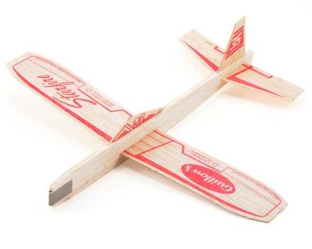
We need to stop for a moment, and think about how we make a glider. We need—
- 5 parts- a canopy, a wing, a fuselage, a rudder, and a stabilizer.
- A location (desk) where you will assemble it.
- A few minutes to put it together.
- A location (down the hallway) where you will test fly it
- And a few minutes of time to test fly it.
- These factors seem a bit like a recipe. In Manufacturing, this list of materials and how they are assembled are referred to as a “Bill of Materials”, or BOM.
Also, the glider parts cost a few dollars to buy, and perhaps, you can sell it to an office mate for a few dollars more. You may need to order the parts, and you want to know how long it will take for new components to show up at your door. You will also want to keep track of how many parts you ordered, where you store the parts, and how many you have on hand. You also may want to reorder parts when your inventory gets below a certain level, so that you can always keep up with demand.
These factors translate to
- Cost price and Sales price,
- Suppliers and lead times,
- Inventory and locations,
- Stockage rules.
We will use all of these factors to define a product. The final road map of the product looks like this:
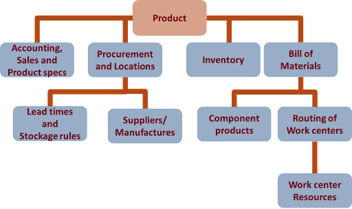
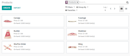
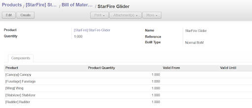
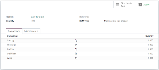
We will create this definition for the final product, as well as all the component products that go into making the final product. Here, you can see the components that go into making a glider.
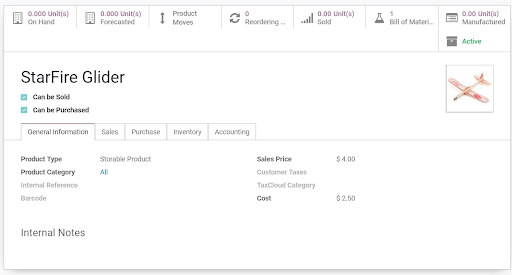
For each product, the definition includes the name of the product, whether it is produced or purchased, the cost and sale price, the parts that make it up ( Bill of Material again), how many in inventory, and when we should reorder it, and the accounting information for purchasing or selling it.
To define the Bill of Material, we will describe the components that are used to make it.
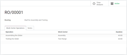
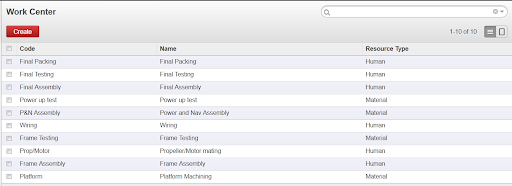
The labor or machine stations where your product is assembled are known as “Work Centers.” In this case, we have defined two different work centers. At the first, you are putting together your glider, and at the second location, you have a space where you can test fly it.
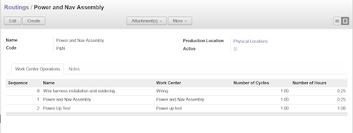
Now, we can add time to assemble your glider at these stations, and define the order in which you will do the work. In building a “Routing” of your work, you are defining the location, time or machine effort, and the order of your assembly. Here, we have defined a “Cycle” of work to take 60 minutes.
By building this model of a proposed product’s assembly system, we can now modify it, and look for optimizations.
We can try variations such as faster machinery, pieces coming to you preassembled, or more staff. You can test your assumptions about production costs prior to ordering equipment or inventory. This alone can save you a lot of time and money.
Some deliverables that may be included might be:
Expected costs, revenue and throughput capability of the complete system.— See example #1
Example #1: Expected costs and revenue calculations.
Let us assume that the company has some data on the time between orders plac ed by customers. Using this data, we can generate an Emperical Distribution Function (EDF) based on the frequency of the data. Next, using tried and true regression techniques, we can fit a number of distributions to the EDF and determine the best fitting distribution.
In the figure below, the blue line represents the raw data and the red line is the best fitting distribution.
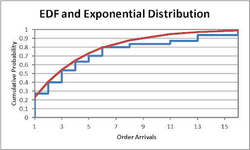
The best fitting distribution using the given data is an Exponential Distribution with the parameter λ = 0.2604. Using the properties of the Exponential Distribution, the mean of the distribution is equal to 1/λ = 3.84 days given that the data was days between order arrivals.
Now lets equate this to the expected cost and revenue. If the expected arrival time is 3.84 days between orders, and using a similar process, we determine the expected number of products in a given order is 25, then we can calculate the expected (E) revenue as:
E[Revenue] = (Revenue per Product)*E[Order Quantity]*(#Business Days/E[order arrival time])
Therefore, if the amount of revenue per product is $20.00 and there are 250 business days in a calendar year, then:
E[Revenue] = $20.00 * 25 * (250/3.84) = $32,55.08
Similar calculations can be used to determine expected costs as well.
Parameters with high sensitivity.
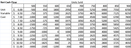
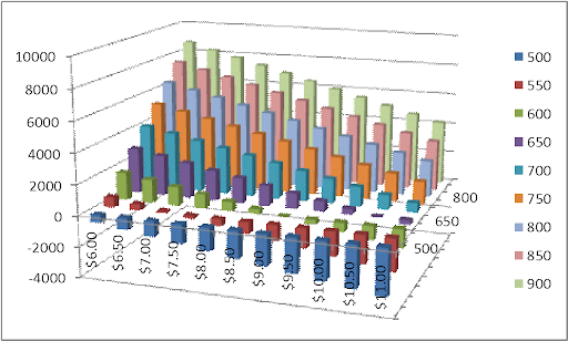
Example #2: Sensitivity Analysis (Variation in Net Cash Flow given changes to Unit Cost and Units Sold):
Optimized manufacturing configuration, and identify possible system constraints.
Example #3: Optimized manufacturing configuration, and identify possible system constraints:
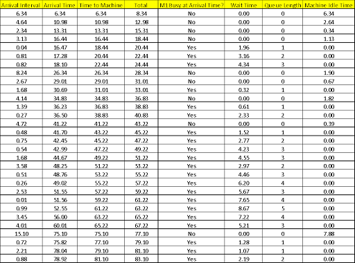
Lets assume that we have a machining process that takes 2 minutes to complete a job from part arrival until completion. Also assume that orders arrive at a rate of 2 orders per minute based on an exponential distribution. The table below represents a simulation of 30 arrivals. Using the arrival data and machine processing time, we can determine valuabl e information that will help the client optimize their process based on certain criteria. For example, we were able to determine not only when the machine was busy, we were also able to calculate idle time. By summing the last column (Machine Idle Time), the machine was idle a total of 23.10 minutes. Given all orders were received and processed within 83.10 minutes, the machine was idle 28% of the time.
How good is this estimate of 28% you ask? Well, the beauty of simulation allows us to re-run this simulation multiple times and determine an average idle time and corresponding standard deviation. We re-ran this simulation 60 times and calculated the following:
Average Machine Idle Time = 13.78%
Standard Deviation of Idle Time = 8.44%
Lastly, we can use the simulation to determine location of possible constraints. Note that the column titled “Queue Length.” Here we can change certain parameters and see the impact on the size of the queue. Also, random breakage times can be introduced and analyzed for downstream impact.
Other things that can be tested for:
Optimized supply chain/vendor selection.
Optimized location ( if lead times differ greatly from place to place).
Reduced costs and risks prior to buying hardware, leasing spaces, or ordering inventory
Prediction of problems or critical issues prior to launch, with possible mitigations.
Confimation of the business plan, by simulating the first XX months or years.
Determine probability distribution functions to model future system performance.
Competitive Analysis
Now, let’s try this for some competitive analysis—Let’s change our scenario a bit.
We have a competitor that makes a small, quiet drone helicopter
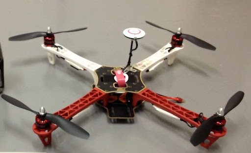
We can use an ERP to simulate how much it costs to make, and how many systems our competitor can make during a day.
We would use the same process described above- We would create a product out of their bill of materials.
- 4 Fiberglass struts,
- 2 Aluminum Carrier platform
- Power distribution board/Battery
- Hardware kit
- Wiring Harness
- 4 Motors
- 4 Propellers
- 3D Robotics Arduino board.
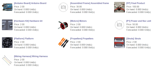
We are making an assumption that there are two major subcomponents in their manufacturing—We think they assemble the frame (all the hardware bits) separately from producing the “brains” as a Power and Nav assembly. We have these broken out as assemblies that will be mated together for the final product.
Next, we can simulate their assembly systems.
We can get information about their address, and then look them up on one of the popular web mapping sites. From here, we can start to get, we can make some assumptions about how big their building is, and how many people work in the office.
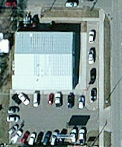
With a little bit of analysis, we can count approximately 20 cars in the parking lot, and 1 truck at a level ground door location. We can assume they have approximately 20 employees, and perhaps 10 people work in assembly.( the balance work may work in administration, sales, shipping/recieiving or other functions).
Doing a bit of measurement, we can guess the building is approximately 4700 square feet as well. Let’s assume ½ of this is availible for manufacturing, so 2350/square feet for assembly
We know that our competitor uses state of the art machine tools and robotic assembly tools that take up approximately 100 square feet. Assuming each machine has one person working with it, and some room between the machines, let’s round this up to 200 square feet each.
These machine tools and robotic assembly stations are set up to each do one task. When we try to build one with the parts in the BOM, we notice it takes 10 steps to assemble and test. We can assume that it may take 10 work stations, one for each step. This also corresponds well to our workforce estimates.
If we have 10 work stations, each at 200 square feet, this calculates to roughly 2000 square feet, and we have figured out that our competitor has only one production line ( There isn’t room for two in this space).
Let’s build the routing of work—Here is the first one for the Power and Nav Assembly:
Now, let’s run this example
We will create a manufacturing order for 25 finished products. We are assuming that we have raw materials in stock. Based on the routings that are set up and the time budgeted for each step, we can get the following results:
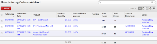
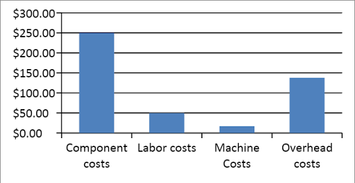
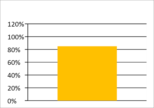
We can sum up the total estimated costs for this manufacturing run and the capacity of the factory used:
We start analyzing the moves and quantities for each component needed to make up the order
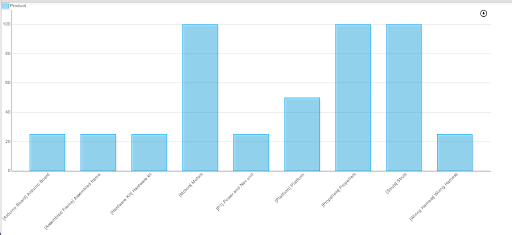
And look for sensitivity based on component lead times, and the min and max ordering quantity for these components.
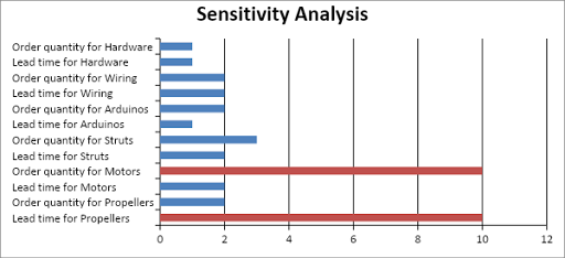
We will repeat this process, changing one thing at a time, and running the different systems in parallel. We will determine probability distribution functions to model future system performance, based on these variations.
By following this process, we can gain a lot of insights.
- Expected costs, revenue and throughput capability of the complete system.
- Parameters with high sensitivity.
- Possible manufacturing configuration.
- Possible supply chain/vendor model
- Analysis of competitor’s advantages ( Supply chain, location, flexibility, costs)
- Benchmarking—You can test your own innovation against this benchmark, and determine risk..
- Examination of competitor to find inflexibility and gaps in the market, and exploit these gaps.


